[본 내용은 밑바닥부터 시작하는 딥러닝을 바탕으로 작성하였습니다.]
4. 신경망 학습
데이터 학습
신경망의 특징은 사람이 아닌 데이터를 중심으로 학습할 수 있다는 점이다. 예를 들어 이전 MNIST 데이터의 image를 보고 사람은 바로 이 숫자가 어떤 것인지 알 수 있지만 컴퓨터가 알아볼 수 있게 적용시킬 수 있는 알고리즘을 생각해내는 것은 어려운 일이다.
따라서 알고리즘을 처음부터 설계하는 방식보다는 데이터를 학습하여 알고리즘을 변형시켜나가는 것이 더 효과적이다. 따라서 이미지 데이터에서 특징을 추출하여 그 패턴을 기계학습 기술로 학습할 수 있다. 보통 이미지를 처리할때는 벡터로 변환한 후 변환된 벡터 데이터를 가지고 supervised learning을 사용한다. (SVM, KNN)
신경망과의 차이점은 사람이 생각한 특징을 먼저 vector로 뽑아내야 하는데 여기서 사람의 판단이 개입된다는 것이다. 하지만 신경망을 구성한다면 해당 특징을 추출해내고 분류해내는 것 모두 기계가 담당할 것이다.
데이터
기계학습 문제는 training data와 test data로 나눠 학습과 실험을 수행하는 것이 일반적이다. 먼저 train data를 사용하여 최적의 매개변수를 찾고 이후 test data를 통해 이 매개변수의 정확성을 측정하는 방식이다.
하지만 train data에 지나치게 최적화된 상태를 오버 피팅이라고 하며 학습의 횟수를 잘 정해 이러한 상태를 피해야 한다.
Loss function
신경망에서 사용하는 Loss function은 최적의 Weight 값을 찾아내기 위해서 사용하는 지표이다.
평균 제곱 오차
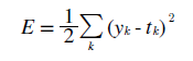
가장 많이 쓰이는 Loss function으로 수식은 위와 같이 나타난다.
import numpy as np

def loss_square(pred, ans):
    return 0.5 * np.sum((pred - ans)**2)

pred_right = np.array([0.1, 0.05, 0.6, 0.0, 0.05, 0.1, 0.0, 0.1, 0.0, 0.0])
pred_fail = np.array([0.1, 0.05, 0.05, 0.0, 0.6, 0.1, 0.0, 0.1, 0.0, 0.0])

ans = np.array([0, 0, 1, 0, 0, 0, 0, 0, 0, 0])

print('[] pred right: ', loss_square(pred_right, ans))
print('[] pred_fail: ', loss_square(pred_fail, ans))
[] pred right:  0.09750000000000003
[] pred_fail:  0.6475
Loss function을 구현한 것이다. pred_? 는 신경망에서 나온 각 정답 확률이고 ans는 index 2가 정답이라는 것을 나타낸다 pred_right은 해당 index에 확률 0.6을 부여하여 정답이 맞게 예측을 했지만 pred_fail은 다른 index의 확률이 더 높다고 판단하였다.
각각의 cost 값을 보게되면 pred_fail의 경우는 cost 값이 크게 나온다. 따라서 이러한 식으로 예측값과 실제 정답의 오차를 구할 수 있다.
교차 엔트로피 오차
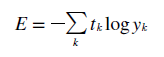
평균 제곱 오차와 같이 교차 엔트로피 오차도 많이 쓰인다. 식은 위와 같다.
import numpy as np
import matplotlib.pyplot as plt

x = np.arange(0.1, 10, 0.00001)
elog = np.log(x)
melog = -np.log(x)

fig = plt.figure()

l1 = fig.add_subplot(1, 2, 1)
l2 = fig.add_subplot(1, 2, 2)

l1.set_xlim(0, 1)
l2.set_xlim(0, 1)

l1.plot(x, elog)
l2.plot(x, melog)
plt.show()
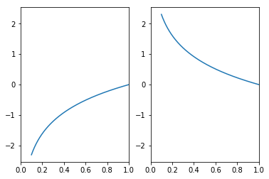
자연 로그의 그래프는 위와 같이 나온다. 위의 식에서 yk는 신경망의 출력, tk는 정답레이블이다.
import numpy as np

def cross_entropy(y, t):
    d = 1e-6
    return -np.sum(t * np.log(y + d))

ans = np.array([0, 0, 1, 0, 0, 0, 0, 0, 0, 0])
pred_right = np.array([0.1, 0.05, 0.6, 0.0, 0.05, 0.1, 0.0, 0.1, 0.0, 0.0])
pred_fail = np.array([0.1, 0.05, 0.0, 0.0, 0.05, 0.1, 0.0, 0.1, 0.0, 0.6])

print('[] pred_right: ', cross_entropy(pred_right, ans))
print('[] pred_fail: ', cross_entropy(pred_fail, ans))
[] pred_right:  0.5108239571007129
[] pred_fail:  13.815510557964274
아까와 같은 input으로 실험을 했을 때 위와 같은 cost 값이 나오게 된다. 손실함수란 결국 내가 예측한 값과 실제 데이터의 정답 사이의 차이를 이끌어내는 함수를 말한다. 그리고 이것을 가장 최소화 시키는 것이 신경망의 정확도를 높이는 방법이다.
그리고 이러한 과정을 위해서 cost function의 값을 최대한 작게하는 가장 알맞은 weight값을 찾으려 미분값을 단서로 해당 매개변수 값을 갱신하는 과정을 반복하게 된다. 이러한 cost 값을 미분하게 되면 그 값은 매개변수의 값의 변화량을 나타내기때문에 음수면 그 매개변수를 양의 방향으로 변화시켜 cost 값을 줄일 수 있다.
따라서 결과적으로 미분 값이 0이면 가중치의 매개변수의 변화량이 더이상 없다는 뜻이기 때문에 갱신은 멈추게 된다.
그리고 cost function을 매개변수의 최적화의 지표로 삼는 이유는 정확도를 지표로 삼았을 시 미분값이 매개변수의 미세한 변화에 따라 연속적으로 움직이지 않기 때문이다.
수치 미분
미분 값은 어떠한 수식에서부터 그 순간의 변화량을 구한 값이다.
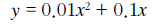
import numpy as np
import matplotlib.pyplot as plt

def func(x):
    return 0.01 * (x ** 2) + (0.1 * x)

x = np.arange(0, 10, 0.01)
y = func(x)

plt.xlabel('x')
plt.ylabel('f(x)')
plt.grid()
plt.plot(x, y)
plt.show()
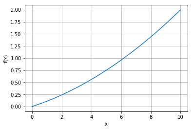
위의 식을 그래프로 나타낸다면 위와 같이 나타난다.
def diff(x):
    h = 1e-4  # 0.0001
    return (func(x + h) - func(x - h)) / (2 * h)


print('[] x == 5 diff: ', diff(5))
[] x == 5 diff: 0.1999999999990898
차분 방법을 이용하여 해당 x값의 기울기를 구할 수 있다.
편미분
앞의 단순한 미분과 달리 미분되는 변수가 2개라는 점이 다르다.
기울기
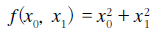
만약 편미분을 동시에 수행한다면 각자의 변피분을 벡터로 정의한 것을 기울기 라고 한다.
import numpy as np

def func(x):
    return np.sum(x ** 2)

def gradient(f, x):
    h = 1e-4
    grad = np.zeros_like(x)

    for i in range(x.size):
        tmp_val = x[i]

        x[i] = tmp_val + h
        fxh1 = f(x)

        x[i] = tmp_val - h
        fxh2 = f(x)

        grad[i] = (fxh1 - fxh2) / (2 * h)
        x[i] = tmp_val

    return grad

x = np.array([1.0, 1.0])
print(gradient(func, x))

x = np.array([2.0, 2.0])
print(gradient(func, x))
[2. 2.]
[4. 4.]
위의 code로 각 점의 편미분 기울기를 구할 수 있다.
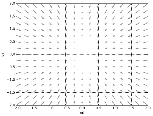
편미분의 기울기 그래프는 위와 같이 나타나는데 사실 기울기라는 것은 가장 낮아지는 방향으로 기울어진다. 더 정확한 표현으로는 기울기가 가리키는 쪽은 각 장소에서 함수의 출력 값을 가장 크게 줄이는 방향 을 뜻한다.
경사법
신경망 역시 최적의 weight 값을 학습 시에 찾아야 한다. 하지만 매개변수의 공간이 넓기 때문에 cost function이 최솟값이 되는 매개변수 값이 무엇인지를 잘 모른다. 그리고 실제 복잡한 함수에서는 기울기 값이 가리키는 방향에 최솟값이 없는 경우가 많다.
이럴 때 경사법 을 사용하게 되는데 이 방식은 현 위치에서 기울어진 방향으로 일정 거리만큼 이동하다가 그 부분에서 기울어진 방향으로 일정거리를 이동 이 과정을 반복하는 방식이 경사법이다.
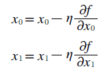
에타 기호는 갱신하는 양을 나타내며 학습률이라고도 한다. 따라서 매개변수 값을 얼마나 갱신하느냐를 정하게 된다.
import numpy as np

def func(x):
    return np.sum(x ** 2)

def gradient(f, x):
    h = 1e-4
    grad = np.zeros_like(x)

    for i in range(x.size):
        tmp_val = x[i]

        x[i] = tmp_val + h
        fxh1 = f(x)

        x[i] = tmp_val - h
        fxh2 = f(x)

        grad[i] = (fxh1 - fxh2) / (2 * h)
        x[i] = tmp_val

    return grad

def gradient_descent(f, init_x, R = 0.01, step = 20):
    x = init_x

    for i in range(0, step):
        grad = gradient(f, x)
        x -= R * grad

    return x

x = np.array([1.0, 1.0])
print(gradient_descent(func, x, 0.01, 1000))
[1.68296736e-09 1.68296736e-09]
경사 하강법을 이용한 최적화된 Weight값을 구하는 code이다.
신경망에서의 기울기
경사 하강법을 신경망 학습에다 적용시켜 최적의 weight 값을 구해야 한다.
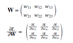
(2, 3) 형태의 가중치(W)가 존재할 때 손실함수는 L, 그리고 경사는 위와 같이 나타난다. (1, 1)에 있는 정보는 w11의 변화량에 따라 L의 변화량이 얼마나 되는지를 나타낸다.
import numpy as np


def func(x):
    return np.sum(x ** 2)

def sigmoid(x):
    return 1 / (1 + np.exp(-x))

def cross_err(y, t):
    if y.ndim == 1:
        t = t.reshape(1, t.size)
        y = y.reshape(1, y.size)

    if t.size == y.size:
        t = t.argmax(axis=1)

    batch_size = y.shape[0]

    return -np.sum(np.log(y[np.arange(batch_size), t] + 1e-7)) / batch_size

def softmax(x):
    if x.ndim == 2:
        x = x.T
        x = x - np.max(x, axis=0)
        y = np.exp(x) / np.sum(np.exp(x), axis=0)
        return y.T

    x = x - np.max(x)
    return np.exp(x) / np.sum(np.exp(x))


def gradient(f, x):
    grad = np.zeros_like(x)
    it = np.nditer(x, flags = ['multi_index'], op_flags = ['readwrite'])
    h = 1e-4

    while not it.finished:
        idx = it.multi_index
        t = x[idx]

        x[idx] = t + h
        fxh1 = f(x)
        print('[] fxh1: ', fxh1)

        x[idx] = t - h
        fxh2 = f(x)
        print('[] fxh2: ', fxh2)

        grad[idx] = (fxh1 - fxh2) / (2 * h)
        x[idx] = t
        it.iternext()

    return grad


class simplenet:
    def __init__(self):
        self.W = np.random.randn(2,3)
#         print(self.W)

    def predict(self, x):
        return np.dot(x, self.W)

    def loss(self, x, t):
        z = self.predict(x)
        y = softmax(z)
        loss = cross_err(y, t)

        return loss


net = simplenet()
#print(net.W.shape)

x = np.array([0.6, 0.1])
t = np.array([0, 0, 1])
print('[] predict: ', net.predict(x))
print('[] Loss: ', net.loss(x, t))
[] predict:  [ 0.94411311 -0.29049154 -0.38802325]
[] Loss:  1.773522958990222
위와 같이 특정 답에 대한 X의 오류를 구할 수 있다.
학습 구현
import numpy as np

class Net:
    def __init__(self, input_size, hidden_size, output_size, R = 0.01):
        self.layer = {}
        self.layer['W1'] = R * np.random.randn(input_size, hidden_size)
        self.layer['b1'] = np.zeros(hidden_size)
        self.layer['W2'] = R * np.random.randn(hidden_size, output_size)
        self.layer['b2'] = np.zeros(output_size)

    def _numerical_gradient_no_batch(f, x):
        h = 1e-4  # 0.0001
        grad = np.zeros_like(x)

        for idx in range(x.size):
            tmp_val = x[idx]
            x[idx] = float(tmp_val) + h
            fxh1 = f(x)

            x[idx] = tmp_val - h
            fxh2 = f(x)
            grad[idx] = (fxh1 - fxh2) / (2*h)

            x[idx] = tmp_val

        return grad


    def numerical_gradient(f, X):
        if X.ndim == 1:
            return _numerical_gradient_no_batch(f, X)
        else:
            grad = np.zeros_like(X)

            for idx, x in enumerate(X):
                grad[idx] = _numerical_gradient_no_batch(f, x)

            return grad

    def sigmoid(self, x):
        return 1 / (1 + np.exp(-x))

    def softmax(self, x):
        if x.ndim == 2:
            x = x.T
            max = np.max(x, 0)

            # nomalization
            x = x - max
            res = np.exp(x) / np.sum(np.exp(x), 0)
            print('[] ndim 2: ', res)
            return res.T

        x = x - np.max(x)
        res = np.exp(x) / np.sum(np.exp(x))
        print('[] ndim 1: ', res)

        return res

    def predict(self, x):
        W1, W2 = self.layer['W1'], self.layer['W2']
        b1, b2 = self.layer['b1'], self.layer['b2']

        L1 = np.dot(x, W1) + b1
        Z1 = self.sigmoid(L1)

        L2 = np.dot(Z1, W2) + b2
        Z2 = self.sigmoid(L2)

        self.res = Z2
        self.res = self.softmax(self.res)

        return self.res

    def cross_entropy_error(y, t):
        if y.ndim == 1:
            t = t.reshape(1, t.size)
            y = y.reshape(1, y.size)

        if t.size == y.size:
            t = t.argmax(axis=1)

        batch_size = y.shape[0]
        return -np.sum(np.log(y[np.arange(batch_size), t] + 1e-7)) / batch_size

    def loss(self, x, t):
        y = self.predict(x)

        return cross_entropy_error(y, t)

    def accuracy(self, pred, t):
        y_argmax = np.argmax(pred, 1)
        t_argmax = np.argmax(t, 1)

        print('[] y_argmax: ', y_argmax)
        print('[] t_argmax: ', t_argmax)

        accu = np.sum(y_argmax == t_argmax) / float(x.shape[0])
        return accu

    def numer_gradient(self, x, t):
        cost = lambda W: self.loss(x, t)

        grads = {}
        grads['W1'] = numer_gradient(cost, self.params['W1'])
        grads['b1'] = numer_gradient(cost, self.params['b1'])
        grads['W2'] = numer_gradient(cost, self.params['W2'])
        grads['b2'] = numer_gradient(cost, self.params['b2'])

        return grads


def main():
    NN = Net(784, 100, 10)


if __name__ == '__main__':
    main()
위에서는 학습을 진행하기 위한 필요한 메소드들을 정리해놓은 class이다. 학습이 진행될수록 grads에는 기울기의 정보가, params 변수에는 weight 값이 저장되게 된다.
import sys
import os
import numpy as np

os.chdir('D:\Machine Learning\deeplearning\example')
from dataset.mnist import *

class TwoLayerNet:
    def __init__(self, input_size, hidden_size, output_size, weight_init_std=0.01):
        self.params = {}
        self.params['W1'] = weight_init_std * np.random.randn(input_size, hidden_size)
        self.params['b1'] = np.zeros(hidden_size)
        self.params['W2'] = weight_init_std * np.random.randn(hidden_size, output_size)
        self.params['b2'] = np.zeros(output_size)

    def predict(self, x):
        W1, W2 = self.params['W1'], self.params['W2']
        b1, b2 = self.params['b1'], self.params['b2']

        a1 = np.dot(x, W1) + b1
        z1 = sigmoid(a1)
        a2 = np.dot(z1, W2) + b2
        y = softmax(a2)

        return y

    def loss(self, x, t):
        y = self.predict(x)

        return cross_entropy_error(y, t)

    def accuracy(self, x, t):
        y = self.predict(x)
        y = np.argmax(y, axis=1)
        t = np.argmax(t, axis=1)

        accuracy = np.sum(y == t) / float(x.shape[0])
        return accuracy

    def numerical_gradient(self, x, t):
        loss_W = lambda W: self.loss(x, t)

        grads = {}
        grads['W1'] = numerical_gradient(loss_W, self.params['W1'])
        grads['b1'] = numerical_gradient(loss_W, self.params['b1'])
        grads['W2'] = numerical_gradient(loss_W, self.params['W2'])
        grads['b2'] = numerical_gradient(loss_W, self.params['b2'])

        return grads

    def gradient(self, x, t):
        W1, W2 = self.params['W1'], self.params['W2']
        b1, b2 = self.params['b1'], self.params['b2']
        grads = {}

        batch_num = x.shape[0]

        # forward
        a1 = np.dot(x, W1) + b1
        z1 = sigmoid(a1)
        a2 = np.dot(z1, W2) + b2
        y = softmax(a2)

        # backward
        dy = (y - t) / batch_num
        grads['W2'] = np.dot(z1.T, dy)
        grads['b2'] = np.sum(dy, axis=0)

        da1 = np.dot(dy, W2.T)
        dz1 = sigmoid_grad(a1) * da1
        grads['W1'] = np.dot(x.T, dz1)
        grads['b1'] = np.sum(dz1, axis=0)

        return grads


(x_train, t_train), (x_test, t_test) = load_mnist(normalize = True, one_hot_label = True)
train_loss_list = []

it = 10
train_size = x_train.shape[0]
total_batch = 100
R = 0.1

net = TwoLayerNet(784, 50, 10)

for i in range(0, it):
    # choice random image index
    batch = np.random.choice(train_size, total_batch)
    x_batch = x_train[batch]
    t_batch = t_train[batch]

    grad = net.numerical_gradient(x_batch, t_batch)
---------------------------------------------------------------------------

NameError                                 Traceback (most recent call last)

<ipython-input-56-dd28aced08c9> in <module>()
     91     t_batch = t_train[batch]
     92
---> 93     grad = net.numerical_gradient(x_batch, t_batch)


<ipython-input-56-dd28aced08c9> in numerical_gradient(self, x, t)
     42
     43         grads = {}
---> 44         grads['W1'] = numerical_gradient(loss_W, self.params['W1'])
     45         grads['b1'] = numerical_gradient(loss_W, self.params['b1'])
     46         grads['W2'] = numerical_gradient(loss_W, self.params['W2'])


NameError: name 'numerical_gradient' is not defined